AlphaZero Explained
01 Jan 2018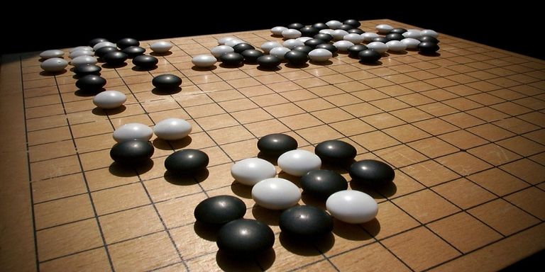
If you follow the AI world, you’ve probably heard about AlphaGo.
The ancient Chinese game of Go was once thought impossible for machines to play. It has more board positions () than there are atoms in the universe. The top grandmasters regularly trounced the best computer Go programs with absurd (10 or 15 stone!) handicaps, justifying their decisions in terms of abstract strategic concepts – joseki, fuseki, sente, tenuki, balance – that they believed computers would never be able to learn.
Demis Hassabis and his team at DeepMind believed otherwise. And they spent three years painstaking years trying to prove this belief; collecting Go data from expert databases, tuning deep neural network architectures, and developing hybrid strategies honed against people as well as machines. Eventually, their efforts culminated in a dizzyingly complex, strategic program they called AlphaGo, trained using millions of hours of CPU and TPU time, able to compete with the best of the best Go players. They set up a match between AlphaGo and grandmaster Lee Sedol … and the rest is history.
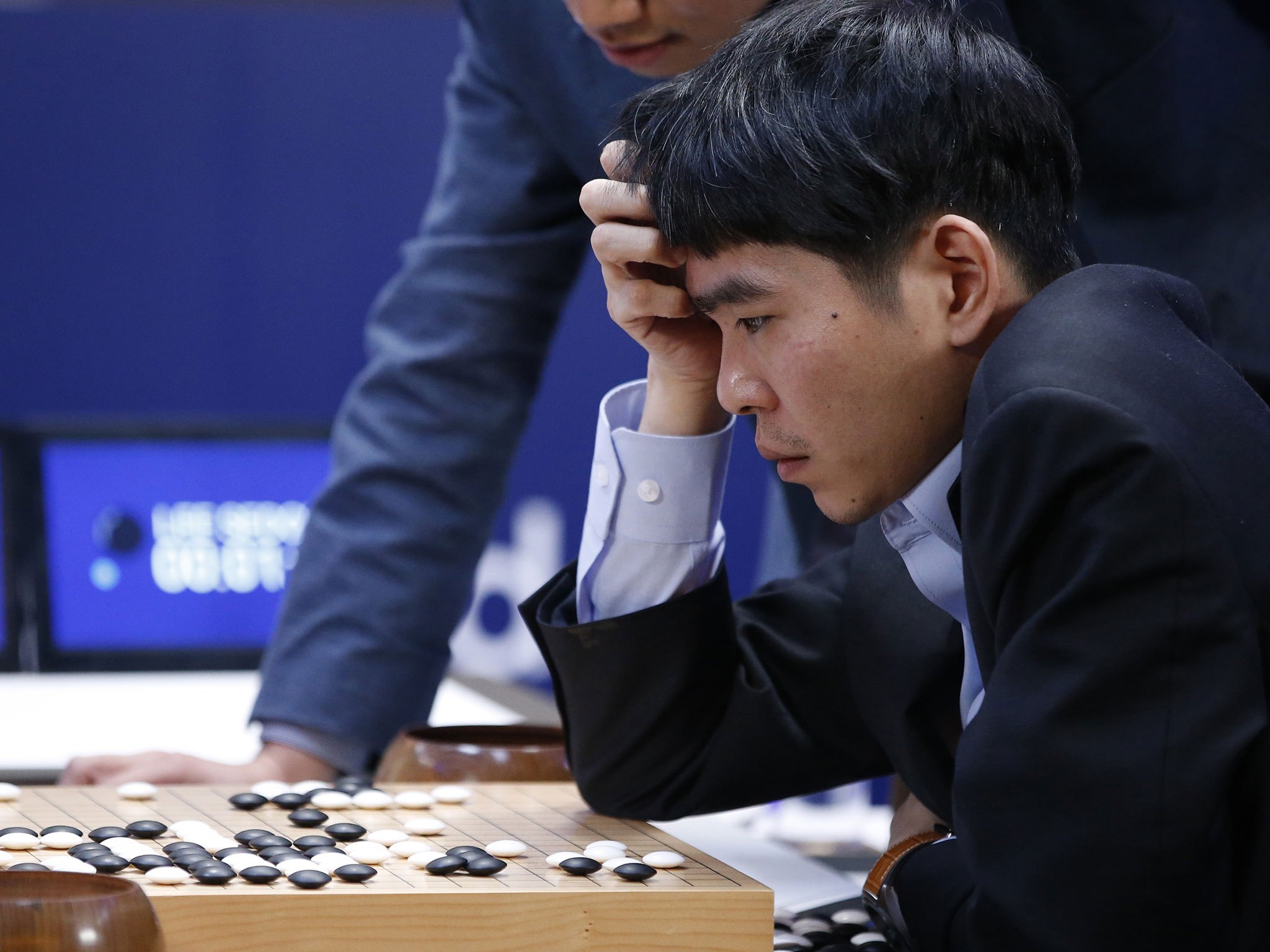
The highly publicized match between Lee Sedol, 9th dan Go grandmaster, and AlphaGo. Google DeepMind’s program won 4 out of 5 games.
But I’m not here to talk about AlphaGo. I’m here to discuss AlphaZero, the algorithm some DeepMind researchers released a year later. The algorithm that uses NO previous information or human-played games whatsoever, starting with nothing but the rules of the game. The algorithm that was able to handily beat the original version of AlphaGo in only four hours (?) of training time. The algorithm that can be applied without modification to chess, Shogi, and almost any other “classical” game with perfect information and no random elements.
If computer programs could feel humilitation, AlphaZero would be making every commercial AI chess or Go program overload with shame. Every single one of them (including the original AlphaGo) uses ridiculously large precomputed tablebases of moves, professional datasets of “well-played games”, and carefully crafted heuristic functions with tons of hacky edge-cases.
“A few years ago I commented to a chess engine developer that the methods of compensating for which side makes the last move in board evaluation seem a bit like slaughtering a chicken under a full moon, and he responded ‘Chess engines slaughter millions of chickens per second‘.” – Bram Cohen
Improving these programs required ekeing out more efficiency from the underlying hardware and making tiny but arcane changes to various interlocking factors and scores. AlphaZero saw the cutthroat, hypercompetitive ecosystem of competitive game-playing, forged through hundreds of thousands of hours of programmer effort and watered with the blood of millions of “slaughtered chickens”, and decided that it was a problem worth spending just four hours on. That’s gotta hurt.
And to add insult to injury, AlphaZero is a radically simple algorithm. It’s so simple that even a lowly blogger like me should be able to explain it and teach YOU how to code it. At least, that’s the idea.
General Game-Playing and DFS
In game theory, rather than reason about specific games, mathematicians like to reason about a special class of games: turn-based, two-player games with perfect information. In these games, both players know everything relevant about the state of the game at any given time. Furthermore, there is no randomness or uncertainty in how making moves affects the game; making a given move will always result in the same final game state, one that both players know with complete certainty. We call games like these classical games.
These are examples of classical games:
whereas these games are not:
- Poker (and most other card games)
- Rock-Paper-Scissors
- The Prisoner’s Dilemma
- Video games like Starcraft
When games have random elements and hidden states, it is much more difficult to design AI systems to play them, although there have been powerful poker and Starcraft AI developed. Thus, the AlphaZero algorithm is restricted to solving classical games only.
In a classical game, because both players have perfect information, every position is either winnable or unwinnable. Either the player who is just about to make a move can win (given that they choose the right move) or they can’t (because no matter what move they make, the game is winnable for the other player). When you add in the possibility of drawing (neither player wins) then there are three possible values for a given state: either it is a guaranteed loss (-1), a guaranteed win (+1), or a guaranteed draw (0).
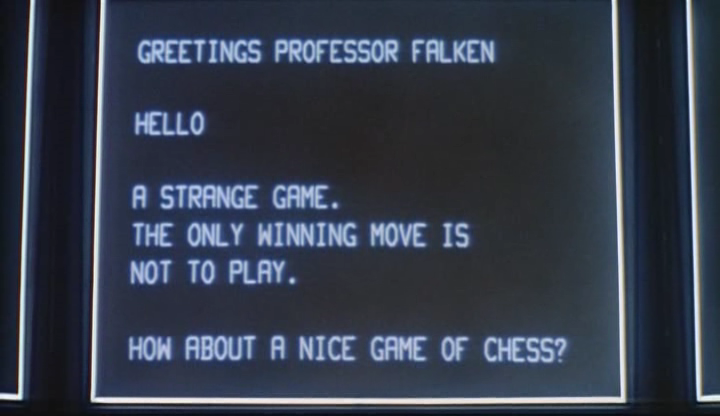
Nuclear warfare: apparently its at most a guaranteed draw. Who would have known?
If this definition makes you shout “Recursion!”, then your instincts are on the right track. In fact, it is easy to determine the value of a game state using a self-referential definition of winnability. We can write some Python code, using my predefined AbstractGame class. Note that we handle the game using general methods, such as make_move(), undo_move(), and over(), that could apply to any game.
from games.games import AbstractGame
from games.tictactoe import TicTacToeGame
from games.chess import ChessGame
from games.gomoku import GomokuGame

r"""
Returns -1 if a game is a guaranteed loss for the player
just about to play, +1 is the game is a guaranteed victory
and 0 for a draw.
"""
def value(game):
    if game.over():
        return -game.score()

    state_values = []
    for move in game.valid_moves():
        game.make_move(move)
        # guaranteed win for P2 is loss for P1, so we flip values
        state_values.append(-value(game))
        game.undo_move()

    # The player always chooses the optimal game state
    # +1 (win) if possible, otherwise draw, then loss
    return max(state_values)
Now, how can we create an AI that always chooses the “best move”? We simply tell the AI to pick a move that results in the lowest resultant score for the opponent. We call this the DFS approach because, to choose a move, we have to do depth-first search on the tree of possible game states.
r"""
Chooses optimal move to play; ideally plays
moves that result in -1 valued states for the opponent
(opponent loses), but will pick draws or opponent victories
if necessary.
"""
def ai_best_move(game):

    action_dict = {}
    for move in game.valid_moves():
        game.make_move(move)
        action_dict[move] = value(game)
        game.undo_move()

    return min(action_dict, key=action_dict.get)
In fact, this simple AI can play tic-tac-toe optimally - it will always either win or draw with anyone it plays.
A simulated game between two AIs using DFS. Since both AIs always pick an optimal move, the game will end in a draw (Tic-Tac-Toe is an example of a game where the second player can always force a draw).
Monte-Carlo Tree Search
So does this mean that we’ve solved all two-player classical games? Not quite. Although the recursion above looks simple, it has to check all possible game states reachable from a given position in order to compute the value of a state. Thus, even though there do exist optimal strategies for complex games like chess and Go, their game trees are so intractably large that it would be impossible to find them.
Branching paths in the game of Go. There are about 150-250 moves on average playable from a given game state.
The reason for the slow progress of DFS is that when estimating the value of a given state in the search, both players must play optimally, choosing the move that gives them the best value, requiring complex recursion. Maybe, instead of making the players choose optimal moves (which is extremely computationally expensive), we can compute the value of a state by making the players choose random moves from there on, and seeing who wins. Or perhaps we could even use cheap computational heuristics to make the players more likely to choose good moves.
This is the basic idea between Monte Carlo Tree Search – use random exploration to estimate the value of a state. We call a single random game a “playout”; if you play 1000 playouts from a given position $X$ and player 1 wins $60\%$ of the time, it’s likely that that position $X$ is better for player 1 than player 2. Thus, we can create a monte_carlo_value() function that estimates the value of a state using a given number of random playouts. Observe how similar this code is to the previous DFS code. The only difference is that instead of iterating through all move possibilities and picking the “best” one, we randomly choose moves.
import random
import numpy as np
from games.games import AbstractGame

def playout_value(game):
    if game.over():
        return -game.score()

    move = random.choice(game.valid_moves())
    game.make_move(move)
    value = -playout_value(game))
    game.undo_move()

    return value

r"""
Finds the expected value of a game by running the specified number
of random simulations.
"""
def monte_carlo_value(game, N=100):
    scores = [playout_value(game) for i in range(0, N)]
    return np.mean(scores)

r"""
Chooses best valued move to play using Monte Carlo Tree search.
"""
def ai_best_move(game):

    action_dict = {}
    for move in game.valid_moves():
        game.make_move(move)
        action_dict[move] = -monte_carlo_value(game)
        game.undo_move()

    return max(action_dict, key=action_dict.get)
Monte Carlo search with a sufficient number of random playouts (usually > 100) can have surprisingly good results on many simple games, including the standard Tic-Tac-Toe. But it is also extremely easy to fool a Monte-Carlo based AI.
To see this, we’re going to have to scale up to a significantly more complicated game: Gomoku. In Gomoku, you win by getting a 5 by 5 row of pieces on a 19 by 19 board. While some positions might be easy to win with against a random opponent, they are utterly undefensible against a competent opponent.
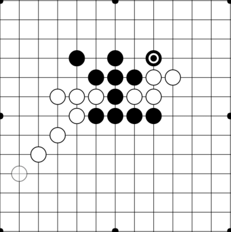
The position above looks good for black from the MCTS perspective. If both white and black are playing randomly, then white only has a chance to pick a game-ending move, while black has a chance to retaliate with a 5-in-a-row choice. But despite this evaluation, any competent player with white would obviously pick the game-ending strategy, so this position should evaluate as overwhelmingly negative for black. In general, MCTS struggles with games with a large number of possible moves.
Upper-Confidence Bounds Applied to Trees (UCT)
One way to fix this problem is to make the move selections within the playouts be more intelligent. Rather than having the move choices within the playouts to be random, we want the opponent to choose their move using some knowledge of what moves are “worth playing”. This is superficially similar to what we did inside our DFS method, where we experimented with every possible move and chose the move with the highest resultant value(). But since computing the true value of a move would be extremely expensive, we instead want to compute a cheap heuristic approximation (heuristic_value()) of the true value of each move, and choose moves within playouts based on this heuristic.
From the perspective of the algorithm, each move is a complete black box – its value unknown –almost like a slot machine with unknown payout probabilities. Some moves might have only a $30\%$ win rate, other moves could have a $70\%$ win rate, but crucially, you don’t know any of this in advance. You need to balance testing the slot machines and recording statistics with actually choosing the best moves. That’s what the UCT algorithm is for: balancing exploration and exploitation in a reasonable way. See this great blog post by Jeff Bradbury for more info.
Thus, we define the heuristic value of a move $V_i$ to be: ,
where:
- $s_i$: the aggregate score after playing move $i$ in all simulations thus far
- $n_i$: the number of plays of move i in all simulations thus far
- $N$: the total number of game states simulated
- $C$: an adjustable constant representating the amount of exploration to allow
The first term in the heuristic encourages exploitation; playing known moves with high values and tend to result in victory. The second term encourages exploration; trying out moves that have a low visit count and updating the statistics so that we have a better knowledge of how valuable/useful these moves are.
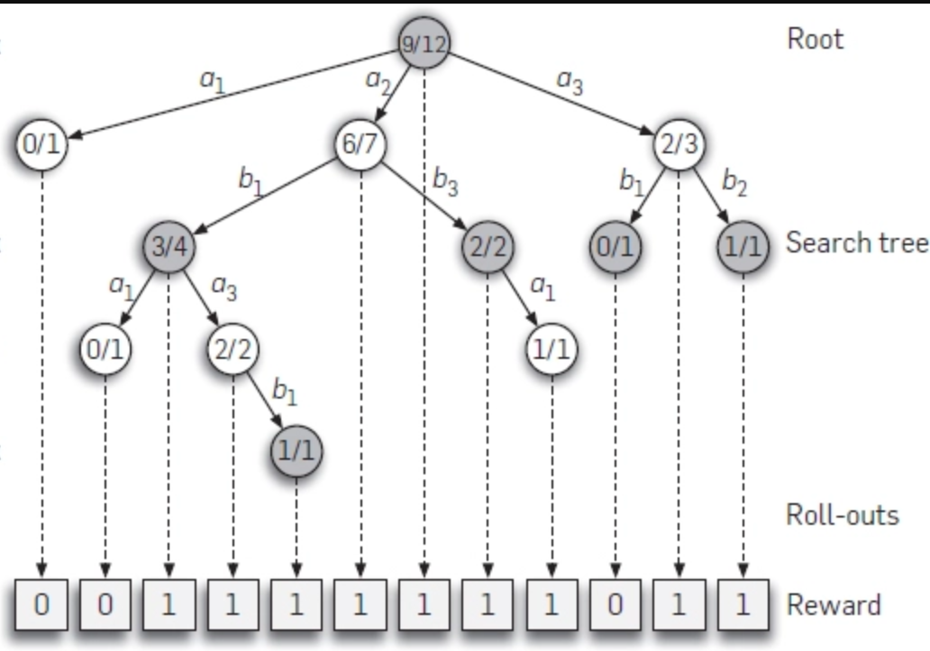
An example search tree using UCT. Note that “promising” moves and branches of the state space are explored more, while unpromising branches that lead to losses are simulated far less.
Whereas the previous two algorithms we worked with, DFS and MCTS, were static, UCT involves learning over time. The first time the UCT algorithm runs, it focuses more on exploring all game states within the playouts (looking a lot like MCTS). But as it collects more and more data, the random playouts become less random and more “heavy”, exploring moves and paths that have already proven to be good choices and ignoring those that haven’t. It uses the statistics collected during simulation about good and bad states, to inform how it computes the winnability of a state. This helps it improve further in a self-reinforcing cycle.
This code shows a simple version of UCT in action. Note that in order to compute moves in a reasonable amount of time, you’d ideally want to parallelize the code to run playouts asynchronously. You can see my efficient, multithreaded implementation of UCT here.
import random
import numpy as np
from utils import hashable
from games.games import AbstractGame

# store statistics
visits = {}
differential = {}

def heuristic_value(game):
    N = visits.get("total", 1)
    Ni = visits.get(hashable(game.state()), 1e-5)
    V = score.get(hashable(game.state()), 0)*1.0/Ni
    return V + C*(np.log(N)/Ni)

# update log for game
def record(game, score):
    visits["total"] = visits.get("total", 1) + 1
    visits[hashable(game.state()] = visits.get(hashable(game.state(), 0) + 1
    differential[hashable(game.state()] = differential.get(hashable(game.state(), 0) + score

def playout_value(game):
    if game.over():
        record(game, -game.score())
        return -game.score()

    action_heuristic_dict = {}
    for move in game.valid_moves():
        game.make_move(move)
        action_heuristic_dict[move] = -heuristic_value(game)
        game.undo_move()
    move = max(action_heuristic_dict, key=action_heuristic_dict.get)
    game.make_move(move)
    value = -playout_value(game)
    game.undo_move()
    record(game, value)

    return value

r"""
Finds the expected value of a game by running the specified number
of UCT simulations. Used in ai_best_move()
"""
def monte_carlo_value(game, N=100):
    scores = [playout(game) for i in range(0, N)]
    return np.mean(scores)
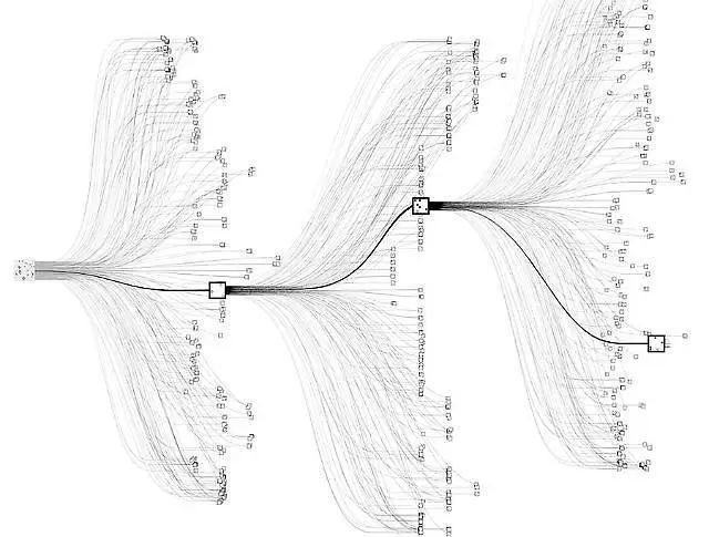
A key component of the success of UCT is how it allows for the construction of lopsided exploration trees. In complex games like chess and Go, there are an incomprehensibly large number of states, but most of them are unimportant because they can only be reached if one or both players play extremely badly. Using UCT, you can avoid exploring out these “useless” states and focus most of your computational energy on simulating games in the interesting portion of the state space, as the diagram below shows.
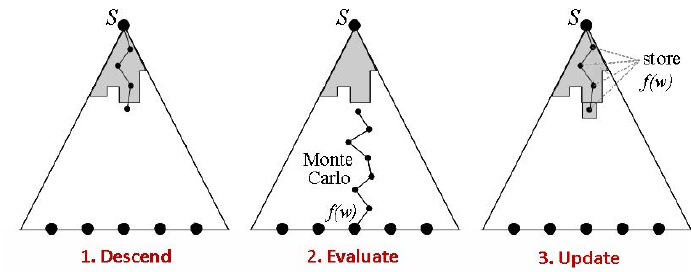
UCT explores the state space of possible moves in a fundamentally asymmetric way.
Deep Learning Heuristic Functions
Given enough playouts, UCT will be able to explore all of the important game positions in any game and determine their values using the Monte Carlo Method. But the amount of playouts needed in games like chess, Go, and Gomoku for this to happen is still computationally infeasible, even with UCT prioritization. Thus, most viable MCTS engines for these games end up exploiting a lot of domain-specific knowledge and heuristics.
To see why, look at the diagram below. The first and second Gomoku games are completely different in terms of the positions of pieces, but the essential components of the “situation” are the same. The differences in piece locations and structure are mostly irrelevant strategically. Yet, to the UCT algorithm, the two games represent different states, and even if UCT has thoroughly “explored” game #1 and knows that it is a +0.2 advantage for black, it has to start from scratch when exploring game #2.
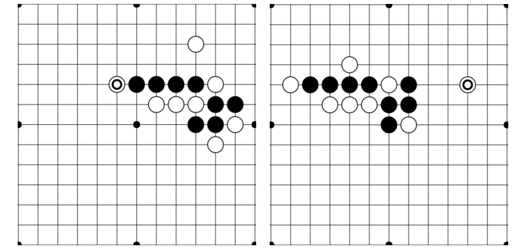
These Gomoku opening games are fundamentally very similar, even though they are shifted and have minor variations in relative piece placement.
Humans have no problem noting the similarities between different game positions and intuitively noting that similar strategies should apply. In fact, rather than memorizing different game states, we tend to do this by default. But how can we train an AI to do the same?
The key here is learning to use deep convolutional neural networks (DCNNs) as fuzzy stores of value. Previous research has shown that DCNNs show success at a wide variety of image tasks, including image classification, scene reconstruction, handwriting recognition, and much more. Crucially, DCNNs are able to learn abstract representations of images; after being shown a few thousand diverse photos of cats, for example, they can learn to classify cats of any angle, location, or color.
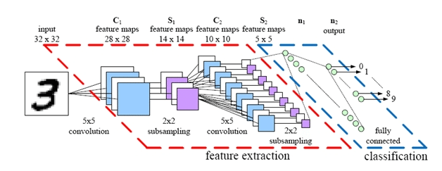
A simple example DCNN architecture. Deep convolutional networks heavily leverage local similarities and structure in images, and may owe their success to being structured similarly to the human optical cortex.
Instead of memorizing a heuristic value for every game state we encounter and putting it in a hashtable, we can train a deep neural network to learn heuristic values from “images” of a game board. The network will remember previous states fairly accurately (assuming we train the DCNN well) but it will also be able to generalize to new, never-before-seen game-states. Sure, because DCNNs are a learning algorithm, the predicted values of states will never be perfect, but that’s OK – we’re just using them as fuzzy heuristics in the search algorithm anyway. All our previous methods were based on exhaustive playouts; adding in a deep neural network gives our models more of the learned “intuition” that human players often leverage.
Here’s some code that creates a simple DCNN in PyTorch (using my torchtrain library to enable Pythonic data loading), designed to predict the value of a given 19 by 19 state in Gomoku.
from torchtrain.modules import TrainableModel

class Net(TrainableModel):

    def __init__(self):

        super(TrainableModel, self).__init__()
        self.conv1 = nn.Conv2d(2, 64, kernel_size=(3, 3), (1, 1))
        self.conv2 = nn.Conv2d(64, 128, kernel_size=(3, 3), (1, 1))
        self.conv3 = nn.Conv2d(128, 128, kernel_size=(3, 3), (1, 1))
        self.conv4 = nn.Conv2d(128, 128, kernel_size=(3, 3), (1, 1))
        self.layer1 = nn.Linear(128, 256)
        self.layer2 = nn.Linear(256, 1)

    def loss(self, data, data_pred):
        Y_pred = data_pred["target"]
        Y_target = data["target"]
        return (F.mse_loss(Y_pred, Y_target))

    def forward(self, data):
        x = data['input']

        # Convolutions mixed with pooling layers
        x = x.view(-1, 2, 19, 19)
        x = F.relu(self.conv1(x))
        x = F.relu(self.conv2(x))
        x = F.max_pool2d(x, (2, 2))
        x = F.relu(self.conv3(x))
        x = F.max_pool2d(x, (2, 2))
        x = F.relu(self.conv4(x))

        x = F.max_pool2d(x, (4, 4))[:, :, 0, 0]
        x = F.dropout(x, p=0.2, training=self.training)

        x = self.layer1(x)
        x = self.layer2(F.tanh(x))

        return {'target': x}
Now, we can modify the record() and heuristic_value() functions to make them train and predict with the neural net, respectively:
# store statistics in DCNN
model = Net()

# update log for game
def record(game, score):
    dataset = [{'input': game.state(), 'target': score}]
    model.fit(dataset, batch_size=1, verbose=False)

def heuristic_value(game):
    dataset = [{'input': game.state(), 'target': None}]
    return model.predict(dataset).mean()
After only two days training with this algorithm, we can achieve near-optimal play (i.e multiple threat sequences followed by a double-threat victory) on 9 by 9 Gomoku with just my single-threaded 2015 Macbook. Using deep learning really does cut down the search time and improve the generality of standard MCTS significantly :)
AlphaZero and The Big Picture
It turns out this is really all there is to the core AlphaZero algorithm, except for a few conceptual and implementation details:
- The neural network architecture used was extremely deep (inspired by the ResNet, which has seen great success on ImageNet and other related computer vision tasks).
- AlphaZero uses a lot of tricks from the computer vision toolbox, including aggressive data augmentation.
- Along with predicting the value of a given state, AlphaZero also tries to predict a probability distribution on the best moves from a given state (to combat overfitting), using a network with a “policy head” and a “value head”. These two measures cross-validate one another to ensure the network is rarely confident about wrong predictions.
- AlphaZero uses a crazy amount of playouts (800 simulations per move) and self-play games (> 100000 games) to learn its value function.
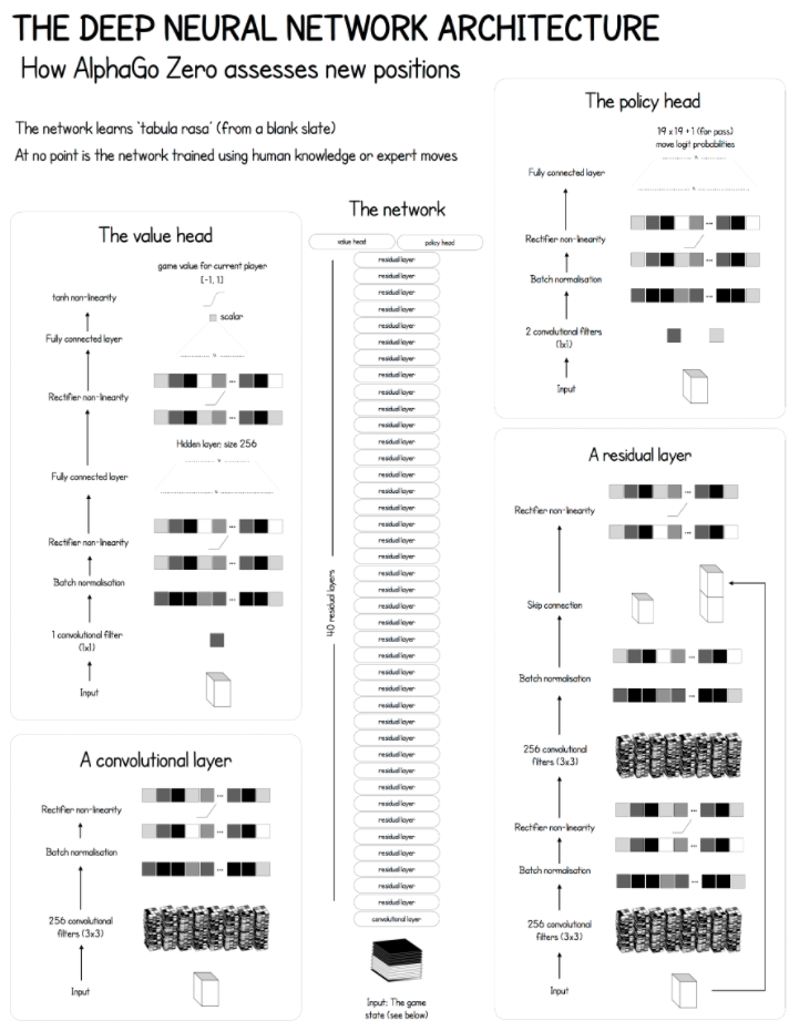
The architecture of AlphaZero as applied to Go. Note that the network layout, especially the input layers, must be game specific, so other games like chess or shogi would require a different DCNN architecture. Diagram from this Medium article.
So why has AlphaZero been so ridiculously successful in so many different domains, given that it is just a straightforward combination of MCTS and UCT with recent deep neural network research?
Some researchers argue that the main strength of AlphaZero was its compute time. The research paper claims that AlphaZero only trained for four hours, but its important to note that this is four hours of training on Google’s most advanced hardware: its prized Tensor Processing Units (or TPUs). Google claims that its TPUs are at least 100x as fast as the highest-end GPUs, and based on extrapolation likely thousands of times faster than the hardware available 2 or 5 years ago. Thus, in a very real sense, it might have been impossible to create AlphaZero before 2017 – the technology just wasn’t there. In fact, if you aren’t Google, it might be impossible to create AlphaZero now, given the many failed/incomplete replication attempts (leela-zero, Roc-Alpha-Go). From that point of view, AlphaZero’s success is more the success of Google’s hardware development team.
But, even if it’s difficult to implement on anything but the fastest hardware, AlphaZero’s design is still brilliant conceptually (certainly much more elegant than the brute-force algorithms that used to dominate top-level chess and Go play), and could provide inspiration for new types of self-learning algorithms. As the deep neural network improves, it makes the MCTS search more efficient, which results in better state valuations to train the deep neural network with – causing a self-reinforcing cycle that can quickly snowball.
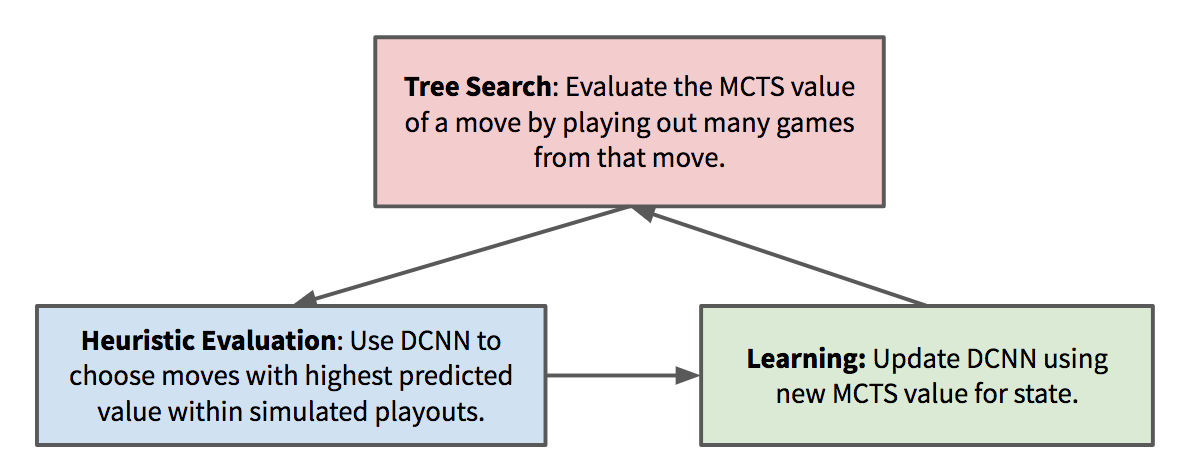
The deep neural network is always playing “catch-up” with the MCTS value predictions. MCTS is in turn improved when it has a better neural network to improve the heuristic value estimations, creating a virtuous cycle of self-improvement. This shares some fundamental similarities with recent research in generative adversarial neural networks (GANs).
Ultimately, the development of AlphaZero is bound to cause a lot of reverbrations in the AI community. Earlier in this post I discussed how shocking AlphaZero’s development was, and its a point I’d like to reiterate. Nobody expected that it would be possible to beat the very best chess and Go engines without any domain knowledge using such an elegant, simple general-purpose algorithm. And nobody could have expected it would have happened this soon. Now it seems like all classical games simple enough for humans to play are also simple enough for computers to solve. What will be the next field that AI eats?