2.1: Linear Regression Using SGD

Linear relationships are some of the simplest possible connections between two variables — yet they show up surprisingly often in nature. If the mass of an object doubles, then the force of gravity on it doubles as well. If the current through a copper wire is halved, the voltage is halved as well.

Linear relationships are also relatively easy to see and characterize in data. Anyone can draw a line through points on a scatterplot. But how do we train a program to do the same?

Data

We’re going to tackle a fairly standard machine learning problem: predicting house prices from their area/square footage.

While the footage a house spans is important to its price (mansions sell for far more than apartments), size isn’t everything. Two houses with the same square footage could have very different prices due to school zoning, amenities, and other factors. Thus, our model of house pricing will likely be highly predictive, but imperfect.

The housing dataset we use is a 200-house subset of data from the Kaggle housing competition. It is hosted in a CSV file on the course github.

We load the CSV in a new Python file using Pandas, then create a scatterplot using Seaborn.

import pandas as pd
import numpy as np
import matplotlib.pyplot as plt
import seaborn as sns
import random

url = "https://raw.githubusercontent.com/nikcheerla/deeplearningschool/master/examples/data/housing.csv"
data = pd.read_csv(url)

area = data["Square Feet (Millions)"]
price = data["Price ($, Millions)"]

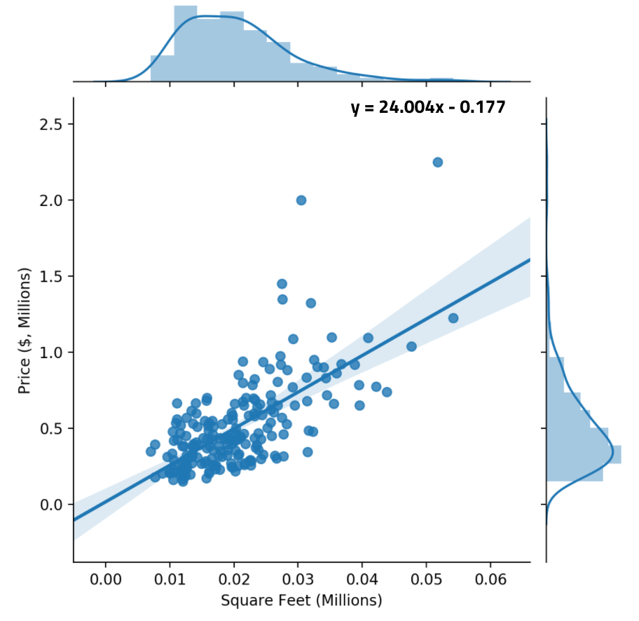
sns.jointplot(area, price);
plt.show()

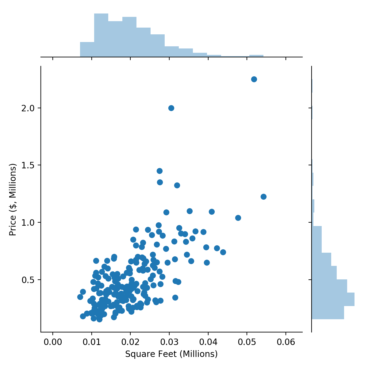
There’s a clear linear relationship between square feet of living area and house price.

Modeling

Now, we develop a linear model to predict house price from house area. We define:

Thus, the price of a house is equal to the area of the house, multiplied by a parameter $m$. For some ideal value of $m$, the resultant line should fit the data points well. We choose $m=1$ as a reasonable initial starting point, and we can find the best value of $m$ through learning.

This linear prediction is represented in a simple predict() function:

M = 1

# Takes in M + numpy array of areas, returns price predictions
def predict(M, input_areas):
	return M*input_areas

Goal Evaluation

Our goal is to accurately predict housing prices. One way to measure how far away our predictions are from the actual values is using the mean-squared error or MSE: the mean of the squared differences between our predictions and the actual values.

Squaring the differences between the actual value and the predicted value ensures that errors in either direction are penalized.

We can write a function evaluate() that computes this mean-squared error, comparing the predicted price for a given value of $M$ with the actual price.

# Evaluates MSE of model y = Mx
def evaluate(M):
	price_predicted = predict(M, area)
	MSE = ((price - price_predicted)**2).mean()
	return MSE

print (evaluate(M=1)) # Error is 0.3258 when M=1

Learning

We could find the optimal value of $m$ by trying all possible values (uniform search), like we did in Section 1.2. But we want the answers found to be accurate and fast — and uniform search necessarily sacrifices one of these constraints. After all, even testing all possible values of $m$ from 0–1, with precision to the fourth decimal place, involves trying 10,000 values!

Clearly, we need to try a different approach.

Gradient Descent

Imagine that you could visualize the loss function or loss landscape for this problem; i.e, the MSE error for every possible model configuration. It might look something like this:

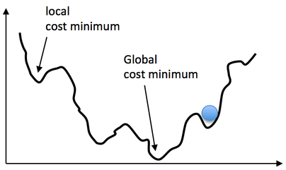
X-axis: possible model configurations (in this case, values of $m$). Y-axis: loss (in this case, MSE).

What you’d note is that, in general, the loss landscape tends to be “smooth” and decreasing until you get to the global cost minimum, which represents the optimal model with least error. There are some “bumps” or local minima that break the pattern, but these tend to be shallow and surpassable. If you rolled a ball down the “hill” that represents the error, the ball would probably end up at the global minimum. Not for certain. But probably.

This inspires an algorithm called gradient descent, in which, like a ball rolling down a hill, we update the model parameters to change in the steepest downhill direction of the error. This works whether there is only one parameter (like in this example, $m$) or when there are many parameters.

1-variable gradient descent.

Multivariable gradient descent, with the two parameters bias and weight. Note how the ball always rolls in the steepest possible downhill direction, eventually arriving at a local (and hopefully global) minimum.

If you’ve taken calculus, you likely recognize what the “steepest downhill direction” is — mathematically, it’s equivalent to the negative of the derivative of the loss or error. (The negative of the gradient when we’re talking about multivariable parameter spaces). Shifting the model to go in the steepest downhill direction would be the equivalent of subtracting the negative derivative of the loss, times some constant. Thus, we can formalize gradient descent for this problem as an update rule:

The initial guess for $m$ is 0, and it keeps on updating based on the gradient. $\alpha$ is the learning rate, and it affects how quickly $m$ changes.

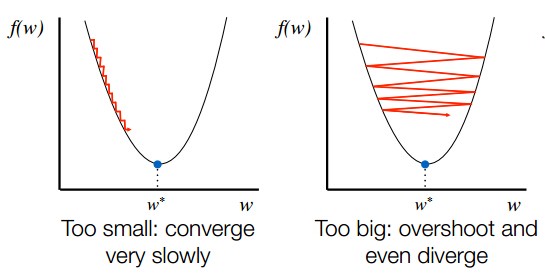
Set $\alpha$ (learning rate) too small and gradient descent will take a long time to reach the minimum. However, set $\alpha$ too large and gradient descent might even diverge.

Stochastic Gradient Descent (SGD)

Most machine learning/deep learning applications use a variant of gradient descent called stochastic gradient descent (SGD), in which instead of updating parameters based on the derivative of the dataset on each step, you update based on the derivative of a randomly chosen sample. The update rule for SGD is similar to gradient descent, but involves random sampling at each iteration:

Not only is this much less computationally taxing, research has shown that the randomness involved in SGD allows it to converge and overcome local minima faster.

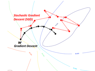
SGD in practice. Note how SGD is more “jerky” and random, but still converges to around the same place as vanilla gradient descent does.

Implementation

To use stochastic gradient descent in our code, we first have to compute the derivative of the loss function with respect to a random sample. The math is shown below:

The per-sample loss is the squared difference between the predicted and actual values; thus, the derivative is easy to compute using the chain rule.

Now, we write a learn() function that chooses a random housing sample and modifies $m$ in the direction of that sample, returning the new (modified) value of $m$. We use a relatively small learning rate of $0.005$ to ensure convergence.

def learn(M):
	j = random.randint(0, len(area) - 1)  # choosing a random sample
	deriv = 2*(M*area[j] - price[j])*M    # derivative calculation
	M = M - 0.005*deriv                   # SGD update step
	return M

Lastly, we create a training loop that applies learn() $2000$ times and shows the convergence to the best value of $m$. Every 100 iterations, we print out the MSE loss, which should ideally decrease as the model becomes better at fitting the data.

for i in range(0, 2000):
	M = learn(M)
	if i % 100 == 0:
		print ("Loss: ", evaluate(M), "(M =", M, ")")

Putting It All Together

import pandas as pd
import numpy as np
import matplotlib.pyplot as plt
import seaborn as sns
import random

url = "https://raw.githubusercontent.com/nikcheerla/deeplearningschool/master/examples/data/housing.csv"
data = pd.read_csv(url)

area = data["Square Feet (Millions)"]
price = data["Price ($, Millions)"]

sns.jointplot(area, price);
plt.show()

M = 1

# Takes in M + numpy array of areas, returns price predictions
def predict(M, input_areas):
	return M*input_areas

# Evaluates MSE of model y = Mx
def evaluate(M):
	price_predicted = predict(M, area)
	MSE = ((price - price_predicted)**2).mean()
	return MSE

print (evaluate(M=1)) # Error is 0.3258 when M=1

def learn(M):
	j = random.randint(0, len(area) - 1) # random sample
	deriv = 2*(M*area[j] - price[j])*M   # derivative calc
	M = M - 0.005*deriv                  # SGD update
	return M

for i in range(0, 2000):
	M = learn(M)
	if i % 100 == 0:
		print ("Loss: ", evaluate(M), "(M =", M, ")")

We run the program, training it to predict house price given house area. It seems to converge on a final slope of around 24, no matter what the initial guess/value of M was.

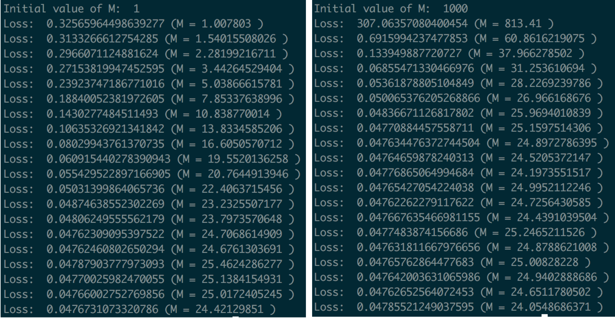
Left: Regression training and loss when m=1 initially. Right: Regression training and loss when m=1000 initially. Note how quickly m drops from its initial value of 1000, compensating for its bad starting point/initial guess.

We compare our predicted value of $m$ to the true line-of-best-fit (linear regression can also be solved analytically to find an mathematically optimal solution). The line-of-best-fit also has an intercept term, so it doesn’t exactly match our solution, but it also achieves a slope of around 24.

Success! We managed to develop a linear model that accurately predicts house prices using Stochastic Gradient Descent.