2.2: Differentiable Circuits And PyTorch

In section 2.1, we delved into the nuts of bolts of linear regression using Python – the linear model, stochastic gradient descent, computing multivariate derivatives for the mean squared error …

Being able to compute linear relationships using gradient descent is certainly important, but there’s more to the story. To create truly useful machine learning pipelines, we need to work with many more variables and far more complex functions. Thus, in this section we go a level of abstraction higher.

Differentiable Circuits

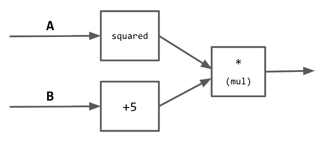
But what does that really mean? The concept of differentiable circuits is key to reasoning about complex machine learning pipelines. (This is a non-standard term, inspired by Karpathy’s Hacker’s Guide To Neural Networks). For example, envision a simple real-valued circuit in which numbers “flow” along edges and interact at intersections.

Circuit that takes in inputs $A$ and $B$ and computes $A^2(B + 5)$.

Tensors, Variables, and Functions in PyTorch

PyTorch is a mathematical framework that allows you to optimize equations using gradient descent. Whereas in regular Python we work with numbers and numpy arrays, with PyTorch we work with multidimensional Tensor and Variable objects that store a history of operations.

For example, here’s how you create a “number” in PyTorch:

import torch

num = torch.FloatTensor([5.0])
num2 = torch.LongTensor([5])

Note that every number (tensor) is actually an array. Furthermore, tensors can have multiple dimensions, representing (for example) stored images or text in a single variable. Tensors can also be of different data types, like FloatTensor or LongTensor, depending on the kind of data they store.

A Variable is a special type of Tensor that also stores a history of operations, and can be differentiated and modified.

import torch
from torch.autograd import Variable

m = Variable(torch.FloatTensor([1.0]), requires_grad=True)
input = Variable(torch.FloatTensor([1.0]), requires_grad=False)

If a variable should be modified — like, for example, the slope parameter $m$ in linear regression — we set the requires_grad flag to True during creation. But some variables, like input data, shouldn’t be mutable at all; thus, we set requires_grad to False for those data types.

Lastly, variables can be modified to create new variables using functions.

import torch
from torch.autograd import Variable
import torch.nn.functional as F

x = Variable(torch.FloatTensor([1.0]), requires_grad=True)
y = Variable(torch.FloatTensor([5.0]), requires_grad=True)
z = (x + y)/(x*y)
w = F.tanh(z)
d = F.mse_loss(w, z)

print (d) # Prints out variable containing 0.1342, MSE between z and w

These operations are mostly self-explanatory, working like regular Python arithmetic operations and math functions, but with the added constraint that variables remember their history. Thus, $d$ is not only the value ($0.1342$) — it is an expression, involving $x, y, w, z$, that evaluates to $0.1342$.

Optimization Using PyTorch

The reason that variable history is important is that it allows us to update variables in order to optimize equations.

For example:

import torch
from torch.autograd import Variable
import torch.nn.functional as F
from torch.optim import SGD, Adadelta

y = Variable(torch.FloatTensor([1.0]), requires_grad=True)
x = Variable(torch.FloatTensor([5.0]), requires_grad=True)
optimizer = SGD([x, y], lr=0.1)

for i in range(0, 100):
	loss = (x-y).abs()	# Minimizes absolute difference
	loss.backward()		# Computes derivatives automatically
	optimizer.step()	# Decreases loss
	optimizer.zero_grad()

print (x)  # Evaluates to 3.0
print (y)  # Evaluates to 3.0 -- optimization successful

You can create an optimizer to compute the derivatives and perform stochastic gradient descent, passing it a list of parameters to optimize and a learning rate. In the above example, we perform SGD to minimize the absolute difference between two variables x and y. Eventually, after 100 steps, the variables both become equal. The fact that PyTorch variables can change to fulfill an equation differentiates them (no pun intended) from regular Python int and float objects.

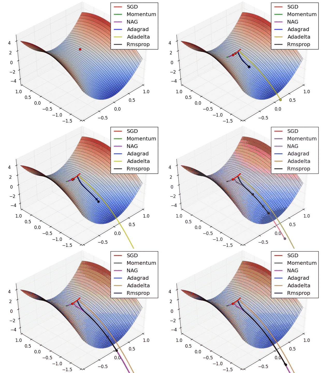
You can even use more advanced optimizers, such as Adadelta. If SGD is like a ball rolling down a hill, then Adadelta is like a person climbing down the same hill. It’s slower and more exploratory, but less likely to overshoot or get stuck; thus, it’s used a lot with more complex deep neural nets.

optimizer = Adadelta((x, y), lr=0.1)

Different optimization algorithms and how they perform on a “saddle point” loss surface. See this post for a full comparison.

We won’t get too much into the details of variables, functions, and optimizers here. But we hope that you have a general familiarity with how PyTorch can be used to speed up and solve optimization problems. Next up: using these new tools to tackle more exotic regression tasks!